Using reactable in #TidyTuesday CHAT dataset - World Energy Production
By Jesús Vélez Santiago in R dataviz
July 23, 2022
Energy production is a crucial aspect of our world’s technological landscape. As we move towards a future of sustainable energy, we need to assess how different countries are progressing in terms of the technologies they adopt for energy production. In this blog post, we’ll dive into some fascinating data obtained from the CHAT dataset, released under CCBY 4.0 and accessed via the National Bureau of Economic Research’s website.
Per the working paper:
We present data on the global diffusion of technologies over time, updating and adding to Comin and Mestieri’s ‘CHAT’ database. We analyze usage primarily based on per capita measures and divide technologies into the two broad categories of production and consumption. We conclude that there has been strong convergence in use of consumption technologies with somewhat slower and more partial convergence in production technologies. This reflects considerably stronger global convergence in quality of life than in income, but we note that universal convergence in use of production technologies is not required for income convergence (only that countries are approaching the technology frontier in the goods and services that they produce).
Preparing the Environment
To analyze the data, we’ll be using various packages in R, including tidyverse for data manipulation, reactable for creating interactive tables, reactablefmtr for enhancing our tables with sparklines and data bars, tidytuesdayR for accessing Tidy Tuesday datasets, htmltools and htmlwidgets for HTML content manipulation and widget creation, countrycode for converting country names and codes, and dataui for data visualization.
library(tidyverse)
library(reactable)
library(reactablefmtr)
library(tidytuesdayR)
library(htmltools)
library(htmlwidgets)
library(countrycode)
library(dataui)
Loading the Data
The dataset we’ll be using is a part of the Tidy Tuesday project, a weekly data project in R for data cleaning, wrangling, and visualization. The dataset, loaded using the tidytuesdayR package, contains information about the adoption of different technologies, specifically those related to energy production.
tuesdata <- tidytuesdayR::tt_load('2022-07-19')

technology <- tuesdata$technology
Here’s a sample of the data we’re working with:
Preparing the Data
In data analysis, the preparation stage is critical to ensure that the data is in the right format and structure for the subsequent analysis. In our case, we’re focusing on energy production technologies and have several steps to transform the raw data into a more digestible format.
General processing
The general processing stage involves filtering and reshaping our dataset. Specifically, we filter the data to focus on energy production, excluding data related to electricity generation capacity. We also perform transformations to adjust the units for electricity consumption and extract information from labels to distinguish between different energy sources and statistics.
This information is then joined with a codelist that provides details such as the country name, continent, and a flag symbol. This enhances our dataset by adding relevant details and ensuring that the data is well-organized for our specific analysis.
technology_processed <- technology |>
  filter(
    group == "Production",
    category == "Energy",
    variable != "electric_gen_capacity"
  ) |>
  mutate(
    value = ifelse(
      test = variable == "elec_cons",
      yes = value / 1e9,
      no = value
    ),
    is_source_energy = str_detect(
      string = label,
      pattern = "Electricity from"
    ),
    is_energy_statistic = !is_source_energy,
    label = label |>
      str_remove(pattern = "Electricity from ") |>
      str_remove(" \\(TWH\\)") |>
      str_to_title()
  ) |>
  left_join(
    y = codelist |>
      select(
        continent,
        country_name = country.name.en,
        iso3c,
        flag = unicode.symbol
      ),
    by = "iso3c"
  ) |>
  mutate(
    country_name = paste(flag, country_name)
  ) |>
  select(
    country_name,
    continent,
    year,
    label,
    variable,
    value,
    is_source_energy,
    is_energy_statistic
  ) |>
  arrange(
    continent,
    country_name,
    variable,
    label,
    year
  )

technology_processed
## # A tibble: 58,976 × 8
## country_name continent year label variable value is_source_energy is_ener…¹
## <chr> <chr> <dbl> <chr> <chr> <dbl> <lgl> <lgl>
## 1 🇦🇴 Angola Africa 2000 Coal elec_coal 0 TRUE FALSE
## 2 🇦🇴 Angola Africa 2001 Coal elec_coal 0 TRUE FALSE
## 3 🇦🇴 Angola Africa 2002 Coal elec_coal 0 TRUE FALSE
## 4 🇦🇴 Angola Africa 2003 Coal elec_coal 0 TRUE FALSE
## 5 🇦🇴 Angola Africa 2004 Coal elec_coal 0 TRUE FALSE
## 6 🇦🇴 Angola Africa 2005 Coal elec_coal 0 TRUE FALSE
## 7 🇦🇴 Angola Africa 2006 Coal elec_coal 0 TRUE FALSE
## 8 🇦🇴 Angola Africa 2007 Coal elec_coal 0 TRUE FALSE
## 9 🇦🇴 Angola Africa 2008 Coal elec_coal 0 TRUE FALSE
## 10 🇦🇴 Angola Africa 2009 Coal elec_coal 0 TRUE FALSE
## # … with 58,966 more rows, and abbreviated variable name ¹is_energy_statistic
Prepare overall values and list of trends
After the general processing, we summarize the data by calculating overall values for each technology and preparing a list of trends for each country. This provides a high-level view of energy production and consumption, allowing us to see which technologies are most prevalent and how these patterns have changed over time.
technology_processed_summarized <- technology_processed |>
  group_by(
    continent,
    country_name,
    variable,
    label
  ) |>
  summarize(
    overall_value = sum(value),
    trend_values = list(value),
    is_energy_statistic = first(is_energy_statistic),
    is_source_energy = first(is_source_energy),
    .groups = "drop"
  )

technology_processed_summarized
## # A tibble: 2,016 × 8
## continent country_name variable label overa…¹ trend…² is_en…³ is_so…⁴
## <chr> <chr> <chr> <chr> <dbl> <list> <lgl> <lgl>
## 1 Africa 🇦🇴 Angola elec_coal Coal 0 <dbl> FALSE TRUE
## 2 Africa 🇦🇴 Angola elec_cons Elec… 54.3 <dbl> TRUE FALSE
## 3 Africa 🇦🇴 Angola elec_gas Gas 19.9 <dbl> FALSE TRUE
## 4 Africa 🇦🇴 Angola elec_hydro Hydro 77.4 <dbl> FALSE TRUE
## 5 Africa 🇦🇴 Angola elec_nuc Nucl… 0 <dbl> FALSE TRUE
## 6 Africa 🇦🇴 Angola elec_oil Oil 16.7 <dbl> FALSE TRUE
## 7 Africa 🇦🇴 Angola elec_renew_other Othe… 0.886 <dbl> FALSE TRUE
## 8 Africa 🇦🇴 Angola elec_solar Solar 0.157 <dbl> FALSE TRUE
## 9 Africa 🇦🇴 Angola elec_wind Wind 0 <dbl> FALSE TRUE
## 10 Africa 🇦🇴 Angola elecprod Gros… 155. <dbl> TRUE FALSE
## # … with 2,006 more rows, and abbreviated variable names ¹overall_value,
## # ²trend_values, ³is_energy_statistic, ⁴is_source_energy
Top energy producers
After the general processing, we summarize the data by calculating overall values for each technology and preparing a list of trends for each country. This provides a high-level view of energy production and consumption, allowing us to see which technologies are most prevalent and how these patterns have changed over time.
top_energy_producers <- technology_processed_summarized |>
  filter(is_energy_statistic) |>
  pivot_wider(
    id_cols = c(continent, country_name),
    names_from = variable,
    values_from = overall_value
  ) |>
  drop_na() |>
  slice_max(
    elecprod,
    n = 50
  )

top_energy_producers
## # A tibble: 50 × 4
##    continent country_name      elec_cons elecprod
##    <chr>     <chr>                 <dbl>    <dbl>
##  1 Americas  🇺🇸 United States    146903.  187739.
##  2 Asia      🇨🇳 China             60290.  105179.
##  3 Europe    🇷🇺 Russia            21097.   61266.
##  4 Asia      🇯🇵 Japan             37901.   45909.
##  5 Europe    🇩🇪 Germany           24227.   28546.
##  6 Americas  🇨🇦 Canada            20517.   28502.
##  7 Asia      🇮🇳 India             14786.   25932.
##  8 Europe    🇫🇷 France            16681.   23549.
##  9 Europe    🇬🇧 United Kingdom    15721.   19685.
## 10 Americas  🇧🇷 Brazil            11272.   16005.
## # … with 40 more rows
Global trends
To provide a comprehensive view of the energy landscape, we also prepare data for analyzing global trends in energy production and consumption. This involves selecting relevant countries from the top energy producers and pivoting the data to make it suitable for trend analysis.
global_trends <- technology_processed_summarized |>
  filter(
    country_name %in% top_energy_producers$country_name,
    is_energy_statistic
  ) |>
  pivot_wider(
    id_cols = c(country_name, continent),
    names_from = variable,
    values_from = trend_values
  ) |>
  inner_join(
    y = top_energy_producers |>
      select(
        country_name,
        overall_consumption = elec_cons,
        overall_production = elecprod
      ),
    by = "country_name"
  ) |>
  arrange(desc(overall_production)) |>
  select(
    country_name,
    continent,
    overall_production,
    overall_consumption,
    production_trends = elecprod,
    consumption_trends = elec_cons
  )

global_trends
## # A tibble: 50 × 6
## country_name continent overall_production overall_cons…¹ produ…² consu…³
## <chr> <chr> <dbl> <dbl> <list> <list>
## 1 🇺🇸 United States Americas 187739. 146903. <dbl> <dbl>
## 2 🇨🇳 China Asia 105179. 60290. <dbl> <dbl>
## 3 🇷🇺 Russia Europe 61266. 21097. <dbl> <dbl>
## 4 🇯🇵 Japan Asia 45909. 37901. <dbl> <dbl>
## 5 🇩🇪 Germany Europe 28546. 24227. <dbl> <dbl>
## 6 🇨🇦 Canada Americas 28502. 20517. <dbl> <dbl>
## 7 🇮🇳 India Asia 25932. 14786. <dbl> <dbl>
## 8 🇫🇷 France Europe 23549. 16681. <dbl> <dbl>
## 9 🇬🇧 United Kingdom Europe 19685. 15721. <dbl> <dbl>
## 10 🇧🇷 Brazil Americas 16005. 11272. <dbl> <dbl>
## # … with 40 more rows, and abbreviated variable names ¹overall_consumption,
## # ²production_trends, ³consumption_trends
Specific trends
Lastly, we prepare data for analyzing specific trends in the use of various energy sources. This involves filtering the data for countries that are among the top energy producers and that have detailed data on energy sources. We also assign colors to each energy source for visual distinction in later stages of our analysis.
Through these steps, we’ve transformed our raw data into a well-structured and detailed dataset that’s ready for in-depth analysis. In the next section, we’ll be delving into data visualization, where we’ll use this prepared data to create an interactive table that presents a comprehensive view of global energy production trends.
specific_trends <- technology_processed_summarized |>
  filter(
    country_name %in% top_energy_producers$country_name,
    is_source_energy
  ) |>
  mutate(
    energy_source_color = case_when(
      label %in% c("Coal", "Gas", "Nuclear", "Oil") ~ "#BB86FC",
      TRUE ~ "#19ffb6"
    )
  ) |>
  arrange(desc(overall_value)) |>
  select(
    country_name,
    energy_source = label,
    overall_value,
    trend_values,
    energy_source_color
  )

specific_trends
## # A tibble: 400 × 5
##    country_name     energy_source overall_value trend_values energy_source_color
##    <chr>            <chr>                 <dbl> <list>       <chr>
##  1 🇨🇳 China         Coal                 71812. <dbl [36]>   #BB86FC
##  2 🇺🇸 United States Coal                 61129. <dbl [36]>   #BB86FC
##  3 🇺🇸 United States Gas                  28412. <dbl [36]>   #BB86FC
##  4 🇺🇸 United States Nuclear              25810. <dbl [36]>   #BB86FC
##  5 🇨🇳 China         Hydro                17547. <dbl [36]>   #19ffb6
##  6 🇮🇳 India         Coal                 16959. <dbl [36]>   #BB86FC
##  7 🇷🇺 Russia        Gas                  15802. <dbl [36]>   #BB86FC
##  8 🇫🇷 France        Nuclear              13903. <dbl [36]>   #BB86FC
##  9 🇨🇦 Canada        Hydro                12479. <dbl [36]>   #19ffb6
## 10 🇧🇷 Brazil        Hydro                10993. <dbl [36]>   #19ffb6
## # … with 390 more rows
Visualizing the Data
Data visualization is an essential tool in the world of data science. It provides a clear, concise way to understand patterns, trends, and insights that might not be immediately apparent in raw, numerical data. To better appreciate the complexities of our data, we’ll now create an interactive table that showcases overall energy production and consumption trends across different countries and continents.
Set global table appearance variables
To start, we need to set up the overall appearance of our table. This involves defining the style elements such as font, color schemes, and border details. In our case, we have chosen a dark theme for our table, with a background color of #121212, border color of #3D3D3D, and text color of white. We’ve also selected the font Atkinson Hyperlegible for its superior readability. The colors for production and consumption data are #4DA1A9 and #ffa630, respectively, providing a clear distinction between the two.
background_color <- "#121212"
border_color <- "#3D3D3D"
text_color <- "white"
font_family <- "Atkinson Hyperlegible"

production_color <- "#4DA1A9"
consumption_color <- "#ffa630"

reactable_theme <- reactableTheme(
    style = list(fontFamily = font_family),
    searchInputStyle = list(background = background_color),
    pageButtonStyle = list(fontSize = 14),
    backgroundColor = background_color,
    color = text_color,
    footerStyle = list(color = text_color, fontSize = 11),
    borderColor = border_color,
    borderWidth = 0.019
)
Create table
With our style elements set, we now move on to creating the actual table. The table is designed to be highly detailed and interactive, providing a wealth of information at a glance while also allowing for deeper dives into specific data points.
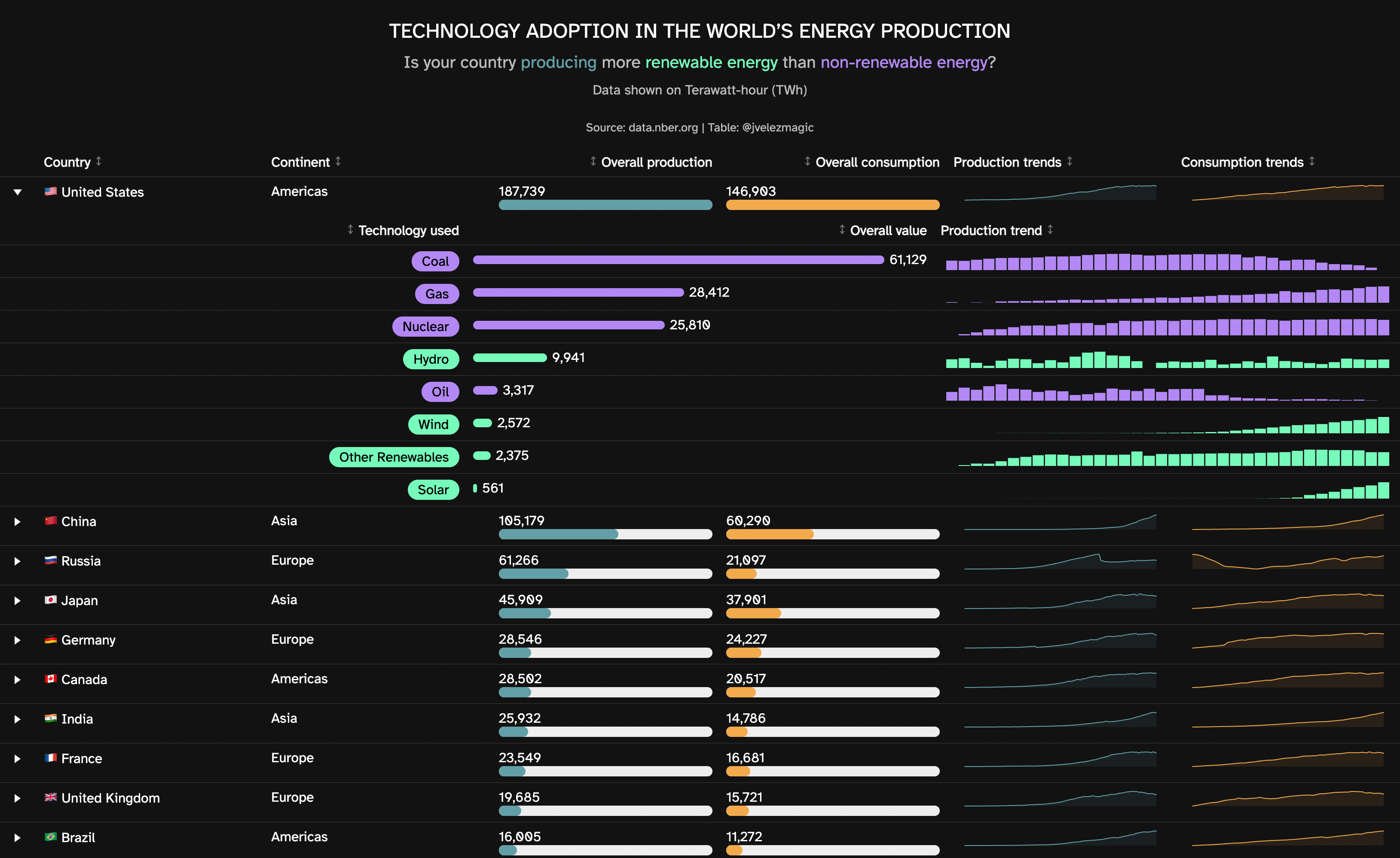
Our table contains columns for country, continent, overall production, overall consumption, and respective trends. To make this data more digestible, we’ve used data bars for overall production and consumption, and sparklines for their trends.
The table also features a details section that, when a specific country is selected, provides additional information about the specific energy technologies used in that country, their overall values, and production trends.
The table is complemented by a text annotation at the top, providing a brief summary and context to the data displayed. It highlights the core question: “Is your country producing more renewable energy than non-renewable energy?”
energy_production_table <- global_trends |>
  reactable(
    theme = reactable_theme,
    columns = list(
      country_name = colDef(
        name = "Country"
      ),
      continent = colDef(
        name = "Continent"
      ),
      overall_production = colDef(
        name = "Overall production",
        cell = data_bars(
          data = select(global_trends, overall_production),
          round_edges = TRUE,
          text_position = "above",
          fill_color = production_color,
          bar_height = 12,
          text_color = text_color,
          number_fmt = scales::label_number(big.mark = ",")
        )
      ),
      overall_consumption = colDef(
        name = "Overall consumption",
        cell = data_bars(
          data = select(global_trends, overall_consumption),
          round_edges = TRUE,
          text_position = "above",
          fill_color = consumption_color,
          bar_height = 12,
          text_color = text_color,
          number_fmt = scales::label_number(big.mark = ",")
        )
      ),
      production_trends = colDef(
        name = "Production trends",
        cell = react_sparkline(
          data = select(global_trends, production_trends),
          line_color = production_color,
          show_area = TRUE
        )
      ),
      consumption_trends = colDef(
        name = "Consumption trends",
        cell = react_sparkline(
          data = select(global_trends, consumption_trends),
          line_color = consumption_color,
          show_area = TRUE
        )
      )
    ),
    showSortable = TRUE,
    showSortIcon = TRUE,
    defaultPageSize = 10,
    details = function(index) {

      current_country <- global_trends$country_name[index]
      current_country_table <- specific_trends |>
        filter(country_name == current_country) |>
        arrange(desc(overall_value))

      current_country_table |>
        reactable(
          theme = reactable_theme,
          columns = list(
            country_name = colDef(
              show = FALSE
            ),
            energy_source = colDef(
              name = "Technology used",
              vAlign = "center",
              headerVAlign = "center",
              align = "right",
              cell = pill_buttons(
                data = current_country_table,
                color_ref = "energy_source_color"
              )
            ),
            overall_value = colDef(
              name = "Overall value",
              cell = data_bars(
                data = current_country_table,
                round_edges = TRUE,
                background = "transparent",
                text_position = "outside-end",
                text_color = text_color,
                fill_gradient = FALSE,
                fill_color_ref = "energy_source_color",
                number_fmt = scales::label_number(big.mark = ","),
                bar_height = 10
              )
            ),
            trend_values = colDef(
              name = "Production trend",
              cell = react_sparkbar(
                data = current_country_table,
                fill_color_ref = "energy_source_color"
              )
            ),
            energy_source_color = colDef(
              show = FALSE
            )
          ),
          showSortable = TRUE,
          showSortIcon = TRUE,
        )
    }
  ) |>
  google_font(
    font_family = font_family
  )

text_annotation <- HTML("
  <div style='vertical-align:middle;text-align:center;background-color:#121212;color:white;padding-top:25px;padding-bottom:4px;font-size:24px;'>
  TECHNOLOGY ADOPTION IN THE WORLD'S ENERGY PRODUCTION
  </div>
  <div style='vertical-align:middle;text-align:center;background-color:#121212;color:#BBBBBB;padding-top:5px;padding-bottom:5px;font-size:20px;'>
  Is your country <span style='color: #4DA1A9'>producing</span> more
  <span style='color: #19ffb6'>renewable energy</span> than
  <span style='color: #BB86FC'>non-renewable energy</span>?
  </div>
  <div style='vertical-align:middle;text-align:center;background-color:#121212;color:#BBBBBB;padding-top:5px;padding-bottom:20px;font-size:16px;'>
  Data shown on Terawatt-hour (TWh)
  </div>
  <div style='vertical-align:middle;text-align:center;background-color:#121212;color:#BBBBBB;padding-top:5px;padding-bottom:15px;font-size:14px;'>
  Source: data.nber.org | Table: @jvelezmagic
  </div>
")

energy_production_table_annotaded <- energy_production_table |>
  prependContent(
    text_annotation
  )


energy_production_table_annotaded
Save table
Finally, we save our table as an HTML file using the save_reactable_test function from the reactablefmtr package. This will allow us to easily share the table with others, or embed it in a webpage for public viewing.
reactablefmtr::save_reactable_test(
  input = energy_production_table_annotaded,
  output = "energy-production-table-annotaded.html"
)
Through effective data visualization, we can better understand the state of global energy production, see which countries are leading the way in renewable energy, and observe how production and consumption trends have changed over time. Stay tuned as we dive deeper into this rich dataset in future posts!
Session info
Show/hide
## ─ Session info ───────────────────────────────────────────────────────────────
##  setting  value
##  version  R version 4.2.1 (2022-06-23)
##  os       macOS Ventura 13.3.1
##  system   aarch64, darwin20
##  ui       X11
##  language (EN)
##  collate  en_US.UTF-8
##  ctype    en_US.UTF-8
##  tz       Europe/Berlin
##  date     2023-05-12
##  pandoc   2.19.2 @ /Applications/RStudio.app/Contents/Resources/app/quarto/bin/tools/ (via rmarkdown)
##
## ─ Packages ───────────────────────────────────────────────────────────────────
##  ! package       * version date (UTC) lib source
##    assertthat      0.2.1   2019-03-21 [2] CRAN (R 4.2.0)
##    backports       1.4.1   2021-12-13 [2] CRAN (R 4.2.0)
##    bit             4.0.4   2020-08-04 [2] CRAN (R 4.2.0)
##    bit64           4.0.5   2020-08-30 [2] CRAN (R 4.2.0)
##  P blogdown        1.16    2022-12-13 [?] CRAN (R 4.2.0)
##  P bookdown        0.34    2023-05-09 [?] CRAN (R 4.2.1)
##    broom           1.0.1   2022-08-29 [2] CRAN (R 4.2.0)
##    bslib           0.4.0   2022-07-16 [2] CRAN (R 4.2.0)
##    cachem          1.0.6   2021-08-19 [2] CRAN (R 4.2.0)
##    cellranger      1.1.0   2016-07-27 [2] CRAN (R 4.2.0)
##    cli             3.4.1   2022-09-23 [2] CRAN (R 4.2.0)
##    colorspace      2.0-3   2022-02-21 [2] CRAN (R 4.2.0)
##  P countrycode   * 1.4.0   2022-05-04 [?] CRAN (R 4.2.0)
##    crayon          1.5.2   2022-09-29 [2] CRAN (R 4.2.0)
##    curl            4.3.2   2021-06-23 [2] CRAN (R 4.2.0)
##  P dataui        * 0.0.1   2023-05-12 [?] Github (timelyportfolio/dataui@39583c6)
##    DBI             1.1.3   2022-06-18 [2] CRAN (R 4.2.0)
##    dbplyr          2.2.1   2022-06-27 [2] CRAN (R 4.2.0)
##    digest          0.6.29  2021-12-01 [2] CRAN (R 4.2.0)
##    dplyr         * 1.0.10  2022-09-01 [2] CRAN (R 4.2.0)
##    ellipsis        0.3.2   2021-04-29 [2] CRAN (R 4.2.0)
##    evaluate        0.16    2022-08-09 [2] CRAN (R 4.2.0)
##    fansi           1.0.3   2022-03-24 [2] CRAN (R 4.2.0)
##    fastmap         1.1.0   2021-01-25 [2] CRAN (R 4.2.0)
##    forcats       * 0.5.2   2022-08-19 [2] CRAN (R 4.2.0)
##    fs              1.5.2   2021-12-08 [2] CRAN (R 4.2.0)
##    gargle          1.2.1   2022-09-08 [2] CRAN (R 4.2.0)
##    generics        0.1.3   2022-07-05 [2] CRAN (R 4.2.0)
##    ggplot2       * 3.3.6   2022-05-03 [2] CRAN (R 4.2.0)
##    glue            1.6.2   2022-02-24 [2] CRAN (R 4.2.0)
##    googledrive     2.0.0   2021-07-08 [2] CRAN (R 4.2.0)
##    googlesheets4   1.0.1   2022-08-13 [2] CRAN (R 4.2.0)
##    gtable          0.3.1   2022-09-01 [2] CRAN (R 4.2.0)
##    haven           2.5.1   2022-08-22 [2] CRAN (R 4.2.0)
##    hms             1.1.2   2022-08-19 [2] CRAN (R 4.2.0)
##  P htmltools     * 0.5.5   2023-03-23 [?] CRAN (R 4.2.0)
##  P htmlwidgets   * 1.6.2   2023-03-17 [?] CRAN (R 4.2.0)
##    httr            1.4.4   2022-08-17 [2] CRAN (R 4.2.0)
##    jquerylib       0.1.4   2021-04-26 [2] CRAN (R 4.2.0)
##    jsonlite        1.8.0   2022-02-22 [2] CRAN (R 4.2.0)
##    knitr           1.40    2022-08-24 [2] CRAN (R 4.2.0)
##    lifecycle       1.0.2   2022-09-09 [2] CRAN (R 4.2.0)
##    lubridate       1.8.0   2021-10-07 [2] CRAN (R 4.2.0)
##    magrittr        2.0.3   2022-03-30 [2] CRAN (R 4.2.0)
##    modelr          0.1.9   2022-08-19 [2] CRAN (R 4.2.0)
##    munsell         0.5.0   2018-06-12 [2] CRAN (R 4.2.0)
##    pillar          1.8.1   2022-08-19 [2] CRAN (R 4.2.0)
##    pkgconfig       2.0.3   2019-09-22 [2] CRAN (R 4.2.0)
##    purrr         * 0.3.4   2020-04-17 [2] CRAN (R 4.2.0)
##    R6              2.5.1   2021-08-19 [2] CRAN (R 4.2.0)
##  P reactable     * 0.4.4   2023-03-12 [?] CRAN (R 4.2.0)
##  P reactablefmtr * 2.0.0   2022-03-16 [?] CRAN (R 4.2.0)
##  P reactR          0.4.4   2021-02-22 [?] CRAN (R 4.2.0)
##    readr         * 2.1.2   2022-01-30 [2] CRAN (R 4.2.0)
##    readxl          1.4.1   2022-08-17 [2] CRAN (R 4.2.0)
##    renv            0.15.5  2022-05-26 [1] CRAN (R 4.2.1)
##    reprex          2.0.2   2022-08-17 [2] CRAN (R 4.2.0)
##    rlang           1.0.6   2022-09-24 [2] CRAN (R 4.2.0)
##    rmarkdown       2.16    2022-08-24 [2] CRAN (R 4.2.0)
##    rstudioapi      0.14    2022-08-22 [2] CRAN (R 4.2.0)
##    rvest           1.0.3   2022-08-19 [2] CRAN (R 4.2.0)
##    sass            0.4.2   2022-07-16 [2] CRAN (R 4.2.0)
##    scales          1.2.1   2022-08-20 [2] CRAN (R 4.2.0)
##    selectr         0.4-2   2019-11-20 [2] CRAN (R 4.2.0)
##  P sessioninfo     1.2.2   2021-12-06 [?] CRAN (R 4.2.0)
##    stringi         1.7.8   2022-07-11 [2] CRAN (R 4.2.0)
##    stringr       * 1.4.1   2022-08-20 [2] CRAN (R 4.2.0)
##    tibble        * 3.1.8   2022-07-22 [2] CRAN (R 4.2.0)
##    tidyr         * 1.2.1   2022-09-08 [2] CRAN (R 4.2.0)
##    tidyselect      1.1.2   2022-02-21 [2] CRAN (R 4.2.0)
##  P tidytuesdayR  * 1.0.2   2022-02-01 [?] CRAN (R 4.2.0)
##    tidyverse     * 1.3.2   2022-07-18 [2] CRAN (R 4.2.0)
##    tzdb            0.3.0   2022-03-28 [2] CRAN (R 4.2.0)
##    usethis         2.1.6   2022-05-25 [2] CRAN (R 4.2.0)
##    utf8            1.2.2   2021-07-24 [2] CRAN (R 4.2.0)
##    vctrs           0.4.2   2022-09-29 [2] CRAN (R 4.2.0)
##    vroom           1.6.0   2022-09-30 [2] CRAN (R 4.2.0)
##    withr           2.5.0   2022-03-03 [2] CRAN (R 4.2.0)
##  P xfun            0.39    2023-04-20 [?] CRAN (R 4.2.0)
##    xml2            1.3.3   2021-11-30 [2] CRAN (R 4.2.0)
##    yaml            2.3.5   2022-02-21 [2] CRAN (R 4.2.0)
##
##  [1] /Users/jvelezmagic/Documents/github/jvelezmagic/renv/library/R-4.2/aarch64-apple-darwin20
##  [2] /Library/Frameworks/R.framework/Versions/4.2-arm64/Resources/library
##
##  P ── Loaded and on-disk path mismatch.
##
## ──────────────────────────────────────────────────────────────────────────────
Details
- Posted on:
- July 23, 2022
- Length:
- 103 minute read, 21752 words
- Tags:
- R dataviz TidyTuesday
- See Also:
- Package: decoupleR
- Iris dataset